Chapter 5 Methods
To generate synthetic populations for each Public Use Microdata Area (PUMA) contained within the Mystic River Watershed area, we used a combination of coding languages (R version 4.2.2 (2022-10-31) and Fortran) and a combination of datasets to generate PUMA-specific constraint tables. Note that the geographic resolution used for these methods is the census tract level.
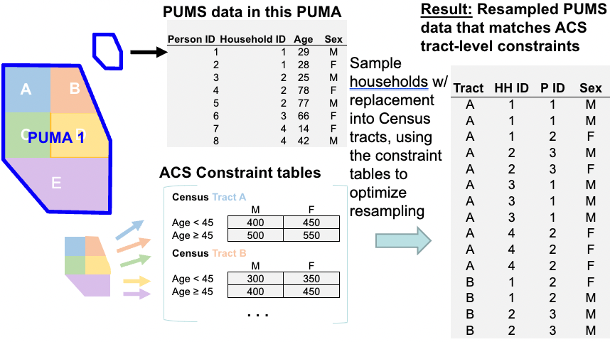
Figure 5.1: Using PUMA and ACS to Generate a Synthetic Population
OVERVIEW:
Obtaining the datasets required:
- Creating lists of census tracts located in each of the 10 PUMAs using R
- Pulling ACS census tract data for each of the 10 PUMA sets of census tracts using R
- Pulling the Public Use Microdata Samples for each PUMA, including person and household variables
The datasets are then cleaned:
- ACS dataset are cleaned and combined in R (with separate runs for each PUMA)
- PUMS data is cleaned and combined in R (with separate runs for each PUMA)
N.B. (1) and (2) above generate output textfiles which can then be read into and implemented in the CO model, which is written in Fortran.
Update a few additional tables:
- Constraining tables information textfile. This file is also an output file with parameters used to reflect different ancestry bins by PUMA.
- Control parameters file with PUMA name, number of constraint cells for that PUMA, and row below (number of constraint cells x 10).
Run with CO_BU.exe, the executable created by compiling Fortran code.
Read the resulting output from the CO work using R.
5.1 Geographic area
There are 21 cities and towns included in the Mystic River Watershed area:
- Burlington
- Lexington
- Belmont
- Watertown
- Arlington
- Winchester
- Woburn
- Reading
- Stoneham
- Medford
- Somerville
- Cambridge
- Boston (East Boston, Charlestown)
- Everett
- Malden
- Melrose
- Wakefield
- Chelsea
- Revere
- Winthrop
- Wilmington
5.2 ACS constraint tables
ACS 5-year (2021) detailed estimates tables for Massachusetts census tracts were obtained.
5.2.1 Race/Ethnicity
- B04006 People Reporting
Ancestry
- Collapsed by town/city: all ancestry groups with more than 1% of the population represented are retained, those with less than 1% are collapsed to ‘other’
- B03001 Hispanic or Latino by Specific Origin
Note that ACS 5-year (2021) detailed estimates tables include People Reporting Single Ancestry, People Reporting Multiple Ancestry, and a combined table of both - People Reporting Ancestry (B04006, used here). In order to approximate the first-ancestry reported, as this is the ancestry included in the PUMS (see section below), we did some re-weighting of the B04006 table variables. In brief, this method was as follows:
For a given PUMA (Public Use Microdata Area) in the set of 10 included PUMAs, and for each census tract within that PUMA, we re-weight all ancestry variables by proceeding across columns.
If true total \(= total_{true}\) and total with multiple ancestries \(= total_{obs}\), and observed population in a given ancestry column for that row \(= Z_{obs}\), then the re-weighted \(Z_{rw}\) is
\[ Z_{rw} = k*Z_{obs} = {\frac{total_{obs}}{total_{true}}}*Z_{obs} \] To round to whole units of persons, we use a probabilistic coin-toss methodology:
Let the probability of rounding up be \(mod(Z_{rw},1)\).
Using the ‘set.seed()’ function in R, generate a random number, \(P\), between 0 and 1.
Then, the rounded number is:
\[ Z_{rw-integer} = Z_{rw}-mod(Z_{rw},1)+P. \] This is helpful, except when the new total, \(total_{new}\) no longer equals \(total_{true}\).To amend this, we apply a ‘fudge factor’: Rank all ancestry columns based on \(Z_{rw_integer}\). Based on the difference between \(total_{true}\) and \(total_{new}\), we adjust the data as needed:
If \(total_{new}-total_{true} = 0\), then do nothing.
If \(total_{new}-total_{true} = total_{diff} > 0\), remove 1 from each of
the top \(n = total_{diff}\) ranked ancestries.
If \(total_{new}-total_{true} = total_{diff} < 0\), add 1 to each of the
top \(n = total_{diff}\) ranked ancestries.
We keep ancestry variables where the proportion of the PUMA of that background equals or exceeds 1%. This means different ancestry variables were included for different PUMAs. The following table provides the list of included ancestries by PUMA.
| PUMA 01300 Ancestries >1% of Total Population |
|---|
| American |
| English |
| French..except.Basque. |
| French.Canadian |
| German |
| Greek |
| Irish |
| Italian |
| Polish |
| Portuguese |
| Scottish |
| Swedish |
| Unclassified.or.not.reported |
| Other |
| PUMA 03306 Ancestries >1% of Total Population |
|---|
| American |
| Arab…Moroccan |
| Brazilian |
| English |
| German |
| Irish |
| Italian |
| Polish |
| Portuguese |
| Unclassified.or.not.reported |
| Other |
| PUMA 00505 Ancestries >1% of Total Population |
|---|
| American |
| Armenian |
| Eastern.European |
| English |
| European |
| French..except.Basque. |
| French.Canadian |
| German |
| Greek |
| Irish |
| Italian |
| Polish |
| Russian |
| Scottish |
| Swedish |
| Unclassified.or.not.reported |
| Other |
| PUMA 03302 Ancestries >1% of Total Population |
|---|
| American |
| English |
| European |
| French..except.Basque. |
| French.Canadian |
| German |
| Irish |
| Italian |
| Polish |
| Russian |
| Scottish |
| Unclassified.or.not.reported |
| Other |
| PUMA 00506 Ancestries >1% of Total Population |
|---|
| American |
| British |
| Eastern.European |
| English |
| European |
| French..except.Basque. |
| German |
| Irish |
| Italian |
| Polish |
| Portuguese |
| Russian |
| Scottish |
| Subsaharan.African…Ethiopian |
| Swedish |
| West.Indian..except.Hispanic.groups….Haitian |
| Unclassified.or.not.reported |
| Other |
| PUMA 00507 Ancestries >1% of Total Population |
|---|
| American |
| Brazilian |
| English |
| European |
| French..except.Basque. |
| French.Canadian |
| German |
| Irish |
| Italian |
| Polish |
| Portuguese |
| Russian |
| West.Indian..except.Hispanic.groups….Haitian |
| Unclassified.or.not.reported |
| Other |
| PUMA 00508 Ancestries >1% of Total Population |
|---|
| American |
| Brazilian |
| English |
| French..except.Basque. |
| French.Canadian |
| German |
| Irish |
| Italian |
| Polish |
| Portuguese |
| Russian |
| Scottish |
| West.Indian..except.Hispanic.groups….Haitian |
| Unclassified.or.not.reported |
| Other |
| PUMA 01000 Ancestries >1% of Total Population |
|---|
| American |
| English |
| French..except.Basque. |
| French.Canadian |
| German |
| Greek |
| Irish |
| Italian |
| Polish |
| Portuguese |
| Russian |
| Scottish |
| Swedish |
| Unclassified.or.not.reported |
| Other |
| PUMA 02800 Ancestries >1% of Total Population |
|---|
| American |
| English |
| French..except.Basque. |
| French.Canadian |
| German |
| Greek |
| Irish |
| Italian |
| Polish |
| Portuguese |
| Scottish |
| Swedish |
| Unclassified.or.not.reported |
| Other |
| PUMA 00503 Ancestries >1% of Total Population |
|---|
| American |
| Armenian |
| English |
| European |
| French..except.Basque. |
| French.Canadian |
| German |
| Greek |
| Irish |
| Italian |
| Polish |
| Russian |
| Scottish |
| Unclassified.or.not.reported |
| Other |
5.2.2 Sex and Age
- B01001 Sex by Age
5.2.5 Householder Age and Tenure
- B25007 Tenure by Age of Householder
5.3 PUMS data
ACS 5-year (2017-2021) Public Use Microdata Sample (PUMS) files for person data and for household data. These data sample approximately 5% of individual responses to the ACS. Full documentation on this data is provided in the PUMS User Guide.
We have downloaded the PUMS data at the highest spatial resolution available: PUMA (Public Use Microdata Area), geographic units developed in the Decennial Census (here, 2010) of approximately 100,000 people per PUMA.
## Rows: 8 Columns: 2
## ── Column specification ────────────────────────────────────────────────────────
## Delimiter: ","
## chr (2): Variable, Explanation
##
## ℹ Use `spec()` to retrieve the full column specification for this data.
## ℹ Specify the column types or set `show_col_types = FALSE` to quiet this message.
## Rows: 5 Columns: 2
## ── Column specification ────────────────────────────────────────────────────────
## Delimiter: ","
## chr (2): Variable, Explanation
##
## ℹ Use `spec()` to retrieve the full column specification for this data.
## ℹ Specify the column types or set `show_col_types = FALSE` to quiet this message.| Variable | Explanation |
|---|---|
| AGEP | Age |
| SEX | Sex |
| ANC1P | Ancestry |
| SCHL | Educational Status |
| SPORDER | Relationship to reference person |
| HISP | Hispanic/Non-Hispanic |
| ID | Identification number |
| SERIALNO | Housing unit/GQ person serial number |
| Variable | Explanation |
|---|---|
| SERIALNO | Housing unit/GQ person serial number |
| TEN | Tenure (owned/rented?) |
| HINCP | Household income |
| ADJINC | Adjusted household income |
| NP | Number of people in house |
5.4 ACS and PUMS Mapping
Because ACS and PUMS variables within tables differ, we create variable mappings between the two datasets for each table. Some mappings are more complex than others (like Ancestry and Hispanic/Latino(a) tables). All are made into factor variables with integers used to indicate categories. The following sections outline the mappings and factors created by constraint variable:
Age (B01001)
Age is a continuous variable in the PUMS dataset. We create age breaks at {0, 17, 24, 34, 44, 64, 200} and make a factor variable (1:6).
Age is a categorical variable in the ACS dataset (as shown above). We use the following mapping to coerce the ACS data into 6 categories that will correspond to the PUMS breaks.
| ACS Category | Recategorization | Corresponding PUMS Factor (continuous integer breaks) |
|---|---|---|
| Under 5 years | 1 | <18 |
| 5-9 years | 1 | <18 |
| 10-14 years | 1 | <18 |
| 15-17 years | 1 | <18 |
| 18 and 19 years | 2 | 18-24 |
| 20 years | 2 | 18-24 |
| 21 years | 2 | 18-24 |
| 22-24 years | 2 | 18-24 |
| 25-29 years | 3 | 25-34 |
| 30-34 years | 3 | 25-34 |
| 35-39 years | 4 | 35-44 |
| 40-44 years | 4 | 35-44 |
| 45-49 years | 5 | 45-64 |
| 50-54 years | 5 | 45-64 |
| 55-59 years | 5 | 45-64 |
| 60 and 61 years | 5 | 45-64 |
| 62-64 years | 5 | 45-64 |
| 65 and 66 years | 6 | 65+ |
| 67-69 years | 6 | 65+ |
| 70-74 years | 6 | 65+ |
| 75-79 years | 6 | 65+ |
| 80-84 years | 6 | 65+ |
| 85 years and over | 6 | 65+ |
Sex (B01001)
The sex variable mappings do not require complex mappings (Male (1) and Female(2)).
Education (B15001)
The education ACS tables do not include the population under 18 years of age. In order for CO_BU.exe to function properly, the person-variables in the estimates_constraints.txt input need to sum to the respective total populations in the census tract. We complete the population for the education section of variables by calculating the remaining under 18 population (using B01001) and include this as a column in the education categories.
| ACS Category | Recategorization | Corresponding PUMS Factor |
|---|---|---|
| Less than 9th grade | 2 | bb N/A (less than 3 years old) |
| Less than 9th grade | 2 | 1 (No schooling completed) |
| Less than 9th grade | 2 | 2 (Nursery school, preschool) |
| Less than 9th grade | 2 | 3 (Kindergarten ) |
| Less than 9th grade | 2 | 4 (Grade 1) |
| Less than 9th grade | 2 | 5 (Grade 2) |
| Less than 9th grade | 2 | 6 (Grade 3) |
| Less than 9th grade | 2 | 7 (Grade 4) |
| Less than 9th grade | 2 | 8 (Grade 5) |
| Less than 9th grade | 2 | 9 (Grade 6) |
| Less than 9th grade | 2 | 10 (Grade 7) |
| Less than 9th grade | 2 | 11 (Grade 8 ) |
| 6th to 12th grade no diploma | 3 | 12 (Grade 9) |
| 7th to 12th grade no diploma | 3 | 13 (Grade 10) |
| 8th to 12th grade no diploma | 3 | 14 (Grade 11) |
| 9th to 12th grade no diploma | 3 | 15 (12th grade - no diploma) |
| High school graduate GED or alternative | 4 | 16 (Regular high school diploma) |
| High school graduate GED or alternative | 4 | 17 (GED or alternative credential) |
| Some college no degree | 5 | 18 (Some college, but less than 1 year) |
| Some college no degree | 5 | 19 (1 or more years of college credit, no degree) |
| Associate degree | 5 | 20 (Associate’s degree) |
| Bachelor degree | 6 | 21 (Bachelor’s degree) |
| Graduate or professional degree | 7 | 22 (Master’s degree) |
| Graduate or professional degree | 7 | 23 (Professional degree beyond a bachelor’s degree) |
| Graduate or professional degree | 7 | 24 (Doctorate degree) |
| Below 18 years Old | 1 | Not included in PUMS |
Householder Age and Household Income (B19037)
Mapping of householder age and household income variables requires setting breaks in PUMS variables (which are continuous integers) that correspond to the ACS categorical values for these variables.Note that householder age from B19037 contains fewer categories than householder age in B25007 (see next subsection).
Additionally, note the added category in the ACS column for B19037 Household Income Mapping. A column of all 0 values is included in the ACS inputs to the estimation_constraints.txt data file in order to provide mapping to the NAs included in the PUMS data.
| ACS Category | Recategorization | Corresponding PUMS Factor (continuous integer breaks) |
|---|---|---|
| Householder under 25 years | 1 | <25 |
| Householder 25-44 years | 2 | 25-44 |
| Householder 45-64 years | 3 | 45-64 |
| Householder 65 years and over | 4 | >64 |
| ACS Category | Recategorization | Corresponding PUMS Factor (continuous integer breaks) |
|---|---|---|
| Less than 10000 | 1 | <10000 |
| 10000-14999 | 2 | 10000-14999 |
| 15000-19999 | 3 | 15000-19999 |
| 20000-24999 | 4 | 20000-24999 |
| 25000-29999 | 5 | 25000-29999 |
| 30000-34999 | 6 | 30000-34999 |
| 35000-39999 | 7 | 35000-39999 |
| 40000-44999 | 8 | 40000-44999 |
| 45000-49999 | 9 | 45000-49999 |
| 50000-59999 | 10 | 50000-59999 |
| 60000-74999 | 11 | 60000-74999 |
| 75000-99999 | 12 | 75000-99999 |
| 100000-124999 | 13 | 100000-124999 |
| 125000-149999 | 14 | 125000-149999 |
| 150000-199999 | 15 | 150000-199999 |
| 200000 or more | 16 | >=200000 |
| NA (Created column where all rows == 0 to match number of PUMS categories) | 17 | NA |
Householder Age and Tenure (B25007)
Mapping of householder tenure requires mapping multiple PUMS tenure categories to individual ACS categories. An additional category is also created for PUMS NA values, and a column of all 0 values is included in the ACS inputs to the estimation_constraints.txt data file in order to provide mapping to the NAs included in the PUMS data.
Additionally, note the added category in the ACS column for B25007 Household Tenure Mapping. A column of all 0 values is included in the ACS inputs to the estimation_constraints.txt data file in order to provide mapping to the NAs included in the PUMS data.
| ACS Category | Recategorization | Corresponding PUMS Factor (continuous integer breaks) |
|---|---|---|
| Householder 15-24 years | 1 | <25 |
| Householder 25-34 years | 2 | 25-34 |
| Householder 35-44 years | 3 | 35-44 |
| Householder 45-54 years | 4 | 45-54 |
| Householder 55-59 years | 5 | 55-59 |
| Householder 60-64 years | 6 | 60-64 |
| Householder 65-74 years | 7 | 65-74 |
| Householder 75-84 years | 8 | 75-84 |
| Householder 85 years and over | 9 | >-85 |
| ACS Category | Recategorization | Corresponding PUMS Factor |
|---|---|---|
| Owner occupied | 1 | 1 (Owned with mortgage or loan (include home equity loans)) |
| Owner occupied | 1 | 2 (Owned free and clear) |
| Renter occupied | 2 | 3 (Rented) |
| Renter occupied | 2 | 4 (Occupied without payment of rent) |
| NA (Created column where all rows == 0 to match number of PUMS categories) | 3 | N/A (GQ/vacant) |
5.5 The Code:
Attention: Before you begin - clone or download the following GitHub Repository: https://github.com/Flannery-BIng/synth_pop
In this repository, you will see two subfolders:
ACRESr
CO_BU
All R scripts are within the ACRESr folder and all Fortran scripts are within the CO_BU folder. Where possible, we have provided example output files and the folder and subfolder structures that will allow you to reproduce our code output.
5.5.1 1. PUMA data
Step 1. Download housing and person level PUMA data here:
https://data.census.gov/app/mdat/ACSPUMS5Y2021
Make sure you select the PUMA variables listed above (see section titled PUMS data).
Step 2. Place the PUMA data in a subfolder of the ACRESr project directory titled ACS_PUMS
5.5.2 2. Prepare ACS data for CO model
This section details the R project structure (hereafter referred to as
ACRESr.proj) implemented prior to running CO_BU.exe.
Step 1. Pulling ACS Data. Run the following code (only need to run 1x): [ACS] - 0 - Grab ACS Data.R
Objectives:
Pull all raw census data using census API calls.
Provide census API key.
Pull all custom functions (custom-functions.R).
Define the PUMAs with census tracts to be included in each.
Run through each individual file that pulls data:
- [ACS] - 0 - i - Ancestry.R
- This script uses a reweight function (process_puma) to get the totals to align with the totals for other categories.
- This script also uses a grab_top_i_percent function to
collapse the number of categories to those contributing at
least i% of the total population.
- [ACS] - 0 - i - Hispanic and Latino.R
- This script also uses a grab_top_i_percent function to
collapse the number of categories to those contributing at
least i% of the total population.
- This script also uses a grab_top_i_percent function to
collapse the number of categories to those contributing at
least i% of the total population.
- [ACS] - 0 - ii - Sex and Age.R
- [ACS] - 0 - iii - Education.R
- [ACS] - 0 - iv - HHage and HHincome.R
- [ACS] - 0 - v - HHage and Tenure.R
- [ACS] - 0 - i - Ancestry.R
Step 2. Output Estimation Constraints and Area List. Run the
following code (run 1x per PUMA, adjusting inputs for lines 16-18):
[ACS] - 1 - combine all.R
Objectives:
- For a given PUMA and its corresponding tracts, pull ACS columns into a table (estimation_constraints) and list all tracts (Area_list).
To do after running:
Copy output from this script into CO_BU/Data.
Copy printed output for calc_pearson.xlsx, and then take the resulting excel column and paste into the constraining_tables_info.txt file in CO_BU/Data.
Go to MA census tract data/ancestry - hispanic B03001/ and copy the resulting hispanic mapping files into the script [PUMS] - 1 - i - Create Ancestry and Hispanic and Latino Mappings.R
Go to MA census tract data/ancestry B04006/ and copy the resulting ancestry mapping files into the script [PUMS] - 1 - i - Create Ancestry and Hispanic and Latino Mappings.R
Step 3. Create Mapped Person and Mapped House files using PUMS data. Run the following code: [PUMS] - 1 - Read in PUMS data.R (run 1x per PUMA, adjusting lines 39 and 40).
Objectives:
For a given PUMA, produce person and household inputs using the PUMA, subset to the variables corresponding to those provided in the ACS table constraints used.
- This code runs all four [PUMS] scripts, creating mappings with [PUMS] - 1 - i - Create Ancestry and Hispanic and Latino Mappings.R, grabbing person data in [PUMS] - 1 - ii - person data.R, household data in [PUMS] - 1 - iii - house data.R, and finally creating the output files in [PUMS] - 1 - iv - convert PUMS to CO.R
To do after running:
- Copy the mapped_person, mapped_house, and house_serials text files from the ACRESr output folder into CO_BU/Data.
5.5.3 3. Bring into the CO model
5.5.3.1 Prepare Data
As described in the R Code, you should have the following files in CO_BU/Data, as listed in CO_filelist.txt (each with the PUMA indicated at the end of the file name, except for CO_random_seednumbers.txt as this does not need to change).
‘Data/mapped_house_PUMA.txt’
‘Data/mapped_person_PUMA.txt’
‘Data/estimation_constraints_PUMA.txt’
‘Data/Area_list_PUMA.txt’
‘Data/constraining_tables_info_PUMA.txt’
‘Data/control_parameters_PUMA.txt’
- Correct line 3 to reflect the name of the folders where you would like the output from CO_BU run to go (see within Estimates and Estimate_Fit). Suggested label: PUMA#.
- Correct lines 7 and 8 to reflect the number of constraint cells (line 7) (see calc_pearson.xlsx for this) and the number of constraint cells scaled by 10x (line 8).
‘Data/CO_random_seednumbers.txt’
5.5.3.2 Run CO_BU.exe
In the terminal, with the directory set to the co-bu-mac folder, run the following:
The make file, make.sh using the code:
cd Code
sh make.sh
Then, in order to run the executable (should see the executable has been created in the co-bu-mac folder):
cd ..
codesign -s - CO_BU
Run the executable:
co-bu-mac % ./CO_BU
5.5.3.3 Read the output and check error
Run [RESULTS] - Read CO output.R:
Calls on each of the individual PUMAs and saves the output from the executable for each as an ‘.rds’ file.
Run [RESULTS] - 2 - Check OTAE.R:
Overall total average error (OTAE): To check the overall total average errors, run this code which pulls all OTAE per household estimates by PUMA and produces a boxplot of the distribution of error by PUMA.
5.5.4 4. Create parcel-level synthetic population
Parcel data can be sourced from state-websites. For Massachusetts, this is a shapefile with a range of available variables (Geographic Information 2025). Before we can proceed with the matching algorithm, we need to do some data preparation.
5.5.4.1 Parcel centroids and PUMAs
Find the centroids of parcels (we did this in GIS, could also do this in R).
01 - [SYNTHPOP] - Joining parcels-tracts-pumas.R
- Joins the geometries (tract to PUMA, parcel centroid to tract)
5.5.4.2 Imputation
Conduct any necessary imputation on parcel data and synthetic population data. Example code for imputation of synthetic population data is available here:
02 - [SYNTHPOP] - Impute Synthpop.R
5.5.4.3 Downscale from tract-level to parcel-level
To downscale further, we need additional data. For this project, we used the MassGIS Property Tax Parcels dataset (Geographic Information 2025). The key variables used from this dataset for this step were:
- Number of rooms
- Year Built
- Total value
We conduct the matching and random allocation in the final ‘synthpop’ code file:
03 - [SYNTHPOP] - Expand MassGIS-Tract to Parcel.R